Reinforcement Learning to Learn MDPs
Introduction
Previous chapters assumed that the agent already knew the structure of the environment. In MDPs, the agent knows everything about the environment and just needs to compute a good plan. In POMDPs, the agent is ignorant of some hidden state but knows how the environment works given this hidden state. Reinforcement Learning (RL) methods apply when the agent doesn’t know the structure of the environment. For example, suppose the agent faces an unknown MDP. Provided the agent observes the reward/utility of states, RL methods will eventually converge on the optimal policy for the MDP. That is, RL eventually learns the same policy that an agent with full knowledge of the MDP would compute.
RL has been one of the key tools behind recent major breakthroughs in AI, such as defeating humans at Go refp:silver2016mastering and learning to play videogames from only pixel input refp:mnih2015human. This chapter applies RL to learning discrete MDPs. It’s possible to generalize RL techniques to continuous state and action spaces and also to learning POMDPs refp:jaderberg2016reinforcement but that’s beyond the scope of this tutorial.
Reinforcement Learning for Bandits
The previous chapter introduced the Multi-Arm Bandit problem. We computed the Bayesian optimal solution to Bandit problems by treating them as POMDPs. Here we apply Reinforcement Learning to Bandits. RL agents won’t perform optimally but they often rapidly converge to the best arm and RL techniques are highly scalable and simple to implement. (In Bandits the agent already knows the structure of the MDP. So Bandits does not showcase the ability of RL to learn a good policy in a complex unknown MDP. We discuss more general RL techniques below).
Outside of this chapter, we use term “utility” (e.g. in the definition of an MDP) rather than “reward”. This chapter follows the convention in Reinforcement Learning of using “reward”.
Softmax Greedy Agent
This section introduces an RL agent specialized to Bandit: a “greedy” agent with softmax action noise. The Softmax Greedy agent updates beliefs about the hidden state (the expected rewards for the arms) using Bayesian updates. Yet instead of making sequential plans that balance exploration (e.g. making informative observations) with exploitation (gaining high reward), the Greedy agent takes the action with highest immediate expected return1 (up to softmax noise).
We measure the agent’s performance on Bernoulli-distributed Bandits by computing the cumulative regret over time. The regret for an action is the difference in expected returns between the action and the objective best action2. In the codebox below, the arms have parameter values (“coin-weights”) of \([0.5,0.6]\) and there are 500 Bandit trials.
///fold:
var cumsum = function (xs) {
  var acf = function (n, acc) { return acc.concat( (acc.length > 0 ? acc[acc.length-1] : 0) + n); }
  return reduce(acf, [], xs.reverse());
  }

///


// Define Bandit problem

// Pull arm0 or arm1
var actions = [0, 1];

// Given a state (a coin-weight p for each arm), sample reward
var observeStateAction = function(state, action){
  var armToCoinWeight = state;
  return sample(Bernoulli({p : armToCoinWeight[action]}))
};


// Greedy agent for Bandits
var makeGreedyBanditAgent = function(params) {
  var priorBelief = params.priorBelief;

  // Update belief about coin-weights from observed reward
  var updateBelief = function(belief, observation, action){
    return Infer({ model() {
      var armToCoinWeight = sample(belief);
      condition( observation === observeStateAction(armToCoinWeight, action))
      return armToCoinWeight;
    }});
  };

  // Evaluate arms by expected coin-weight
  var expectedReward = function(belief, action){
    return expectation(Infer( { model() {
      var armToCoinWeight = sample(belief);
      return armToCoinWeight[action];
    }}))
  }

  // Choose by softmax over expected reward
  var act = dp.cache(
    function(belief) {
      return Infer({ model() {
        var action = uniformDraw(actions);
        factor(params.alpha * expectedReward(belief, action))
        return action;
      }});
    });

  return { params, act, updateBelief };
};

// Run Bandit problem
var simulate = function(armToCoinWeight, totalTime, agent) {
  var act = agent.act;
  var updateBelief = agent.updateBelief;
  var priorBelief = agent.params.priorBelief;

  var sampleSequence = function(timeLeft, priorBelief, action) {
    var observation = (action !== 'noAction') &&
                      observeStateAction(armToCoinWeight, action);
    var belief = ((action === 'noAction') ? priorBelief :
                  updateBelief(priorBelief, observation, action));
    var action = sample(act(belief));

    return (timeLeft === 0) ? [action] :
           [action].concat(sampleSequence(timeLeft-1, belief, action));
  };
  return sampleSequence(totalTime, priorBelief, 'noAction');
};


// Agent params
var alpha = 30
var priorBelief = Infer({  model () {
  var p0 = uniformDraw([.1, .3, .5, .6, .7, .9]);
  var p1 = uniformDraw([.1, .3, .5, .6, .7, .9]);
  return { 0:p0, 1:p1};
} });

// Bandit params
var numberTrials = 500;
var armToCoinWeight = { 0: 0.5, 1: 0.6 };

var agent = makeGreedyBanditAgent({alpha, priorBelief});
var trajectory = simulate(armToCoinWeight, numberTrials, agent);

// Compare to random agent
var randomTrajectory = repeat(
    numberTrials,
    function(){return uniformDraw([0,1]);}
);

// Compute agent performance
var regret = function(arm) {
  var bestCoinWeight = _.max(_.values(armToCoinWeight))
  return bestCoinWeight - armToCoinWeight[arm];
};

var trialToRegret = map(regret,trajectory);
var trialToRegretRandom = map(regret, randomTrajectory)
var ys = cumsum( trialToRegret)

print('Number of trials: ' + numberTrials);
print('Total regret: [GreedyAgent, RandomAgent]  ' +
      sum(trialToRegret) + ' ' + sum(trialToRegretRandom))
print('Arms pulled: ' +  trajectory);

viz.line(_.range(ys.length), ys, {xLabel:'Time', yLabel:'Cumulative regret'});
How well does the Greedy agent do? It does best when the difference between arms is large but does well even when the arms are close. Greedy agents perform well empirically on a wide range of Bandit problems refp:kuleshov2014algorithms and if their noise decays over time they can achieve asymptotic optimality. In contrast to the optimal POMDP agent from the previous chapter, the Greedy Agent scales well in both number of arms and trials.
Exercises:
- Modify the code above so that it’s easy to repeatedly run the same agent on the same Bandit problem. Compute the mean and standard deviation of the agent’s total regret averaged over 20 episodes on the Bandit problem above. Use WebPPL’s library functions.
- Set the softmax noise to be low. How well does the Greedy Softmax agent do? Explain why. Keeping the noise low, modify the agent’s priors to be overly “optimistic” about the expected reward of each arm (without changing the support of the prior distribution). How does this optimism change the agent’s performance? Explain why. (An optimistic prior assigns a high expected reward to each arm. This idea is known as “optimism in the face of uncertainty” in the RL literature.)
- Modify the agent so that the softmax noise is low and the agent has a “bad” prior (i.e. one that assigns a low probability to the truth) that is not optimistic. Will the agent always learn the optimal policy (eventually?) If so, after how many trials is the agent very likely to have learned the optimal policy? (Try to answer this question without doing experiments that take a long time to run.)
Posterior Sampling
Posterior sampling (or “Thompson sampling”) is the basis for another algorithm for Bandits. This algorithm generalizes to arbitrary discrete MDPs, as we show below. The Posterior-sampling agent updates beliefs using standard Bayesian updates. Before choosing an arm, it draws a sample from its posterior on the arm parameters and then chooses greedily given the sample. In Bandits, this is similar to Softmax Greedy but without the softmax parameter \(\alpha\).
Exercise: Implement Posterior Sampling for Bandits by modifying the code above. (You only need to modify the
actfunction.) Compare the performance of Posterior Sampling to Softmax Greedy (using the value for \(\alpha\) in the codebox above). You should vary thearmToCoinWeightparameter and the number of arms. Evaluate each agent by computing the mean and standard deviation of rewards averaged over many trials. Which agent is better overall and why?
RL algorithms for MDPs
The RL algorithms above are specialized to Bandits and so they aren’t able to learn an arbitrary MDP. We now consider algorithms that can learn any discrete MDP. There are two kinds of RL algorithm:
-
Model-based algorithms learn an explicit representation of the MDP’s transition and reward functions. These representations are used to compute a good policy.
-
Model-free algorithms do not explicitly represent or learn the transition and reward functions. Instead they explicitly represent either a value function (i.e. an estimate of the \(Q^*\)-function) or a policy.
The best known RL algorithm is Q-learning, which works both for discrete MDPs and for MDPs with high-dimensional state spaces (where “function approximation” is required). Q-learning is a model-free algorithm that directly learns the expected utility/reward of each action under the optimal policy. We leave as an exercise the implementation of Q-learning in WebPPL. Due to the functional purity of WebPPL, a Bayesian version of Q-learning is more natural and in the spirit of this tutorial. See, for example “Bayesian Q-learning” refp:dearden1998bayesian and this review of Bayesian model-free approaches refp:ghavamzadeh2015bayesian.
Posterior Sampling Reinforcement Learning (PSRL)
Posterior Sampling Reinforcemet Learning (PSRL) is a model-based algorithm that generalizes posterior-sampling for Bandits to discrete, finite-horizon MDPs refp:osband2016posterior. The agent is initialized with a Bayesian prior distribution on the reward function \(R\) and transition function \(T\). At each episode the agent proceeds as follows:
- Sample \(R\) and \(T\) (a “model”) from the distribution. Compute the optimal policy for this model and follow it until the episode ends.
- Update the distribution on \(R\) and \(T\) on observations from the episode.
How does this agent efficiently balances exploration and exploitation to rapidly learn the structure of an MDP? If the agent’s posterior is already concentrated on a single model, the agent will mainly “exploit”. If the agent is uncertain over models, then it will sample various different models in turn. For each model, the agent will visit states with high reward on that model and so this leads to exploration. If the states turn out not to have high reward, the agent learns this and updates their beliefs away from the model (and will rarely visit the states again).
The PSRL agent is simple to implement in our framework. The Bayesian belief-updating re-uses code from the POMDP agent: \(R\) and \(T\) are treated as latent state and are observed every state transition. Computing the optimal policy for a sampled \(R\) and \(T\) is equivalent to planning in an MDP and we can re-use our MDP agent code.
We run the PSRL agent on Gridworld. The agent knows \(T\) but does not know \(R\). Reward is known to be zero everywhere but a single cell of the grid. The actual MDP is shown in Figure 1, where the time-horizon is 8 steps. The true reward function is specified by the variable trueLatentReward (where the order of the rows is the inverse of the displayed grid). The displays shows the agent’s trajectory on each episode (where the number of episodes is set to 10).
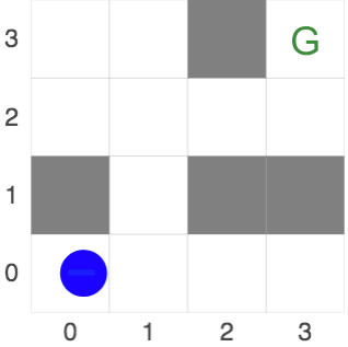
Figure 1: True latent reward for Gridworld below. Agent receives reward 1 in the cell marked “G” and zero elsewhere.
///fold:

// Construct Gridworld (transitions but not rewards)
var ___ = ' ';

var grid = [
  [ ___, ___, '#', ___],
  [ ___, ___, ___, ___],
  [ '#', ___, '#', '#'],
  [ ___, ___, ___, ___]
];

var pomdp = makeGridWorldPOMDP({
  grid,
  start: [0, 0],
  totalTime: 8,
  transitionNoiseProbability: .1
});

var transition = pomdp.transition

var actions = ['l', 'r', 'u', 'd'];

var utility = function(state, action) {
  var loc = state.manifestState.loc;
  var r = state.latentState.rewardGrid[loc[0]][loc[1]];

  return r;
};


// Helper function to generate agent prior
var getOneHotVector = function(n, i) {
  if (n==0) {
    return [];
  } else {
    var e = 1*(i==0);
    return [e].concat(getOneHotVector(n-1, i-1));
  }
};
///

var observeState = function(state) {
  return utility(state);
};


var makePSRLAgent = function(params, pomdp) {
  var utility = params.utility;

  // belief updating: identical to POMDP agent from Chapter 3c
  var updateBelief = function(belief, observation, action){
    return Infer({ model() {
      var state = sample(belief);
      var predictedNextState = transition(state, action);
      var predictedObservation = observeState(predictedNextState);
      condition(_.isEqual(predictedObservation, observation));
      return predictedNextState;
    }});
  };

  // this is the MDP agent from Chapter 3a
  var act = dp.cache(
    function(state) {
      return Infer({ model() {
        var action = uniformDraw(actions);
        var eu = expectedUtility(state, action);
        factor(1000 * eu);
        return action;
      }});
    });

  var expectedUtility = dp.cache(
    function(state, action) {
      return expectation(
        Infer({ model() {
          var u = utility(state, action);
          if (state.manifestState.terminateAfterAction) {
            return u;
          } else {
            var nextState = transition(state, action);
            var nextAction = sample(act(nextState));
            return u + expectedUtility(nextState, nextAction);
          }
        }}));
    });

  return { params, act, expectedUtility, updateBelief };
};


var simulatePSRL = function(startState, agent, numEpisodes) {
  var act = agent.act;
  var updateBelief = agent.updateBelief;
  var priorBelief = agent.params.priorBelief;

  var runSampledModelAndUpdate = function(state, priorBelief, numEpisodesLeft) {
    var sampledState = sample(priorBelief);
    var trajectory = simulateEpisode(state, sampledState, priorBelief, 'noAction');
    var newBelief = trajectory[trajectory.length-1][2];
    var newBelief2 = Infer({ model() {
      return extend(state, {latentState : sample(newBelief).latentState });
    }});
    var output = [trajectory];

    if (numEpisodesLeft <= 1){
      return output;
      } else {
      return output.concat(runSampledModelAndUpdate(state, newBelief2,
                                                    numEpisodesLeft-1));
    }
  };

  var simulateEpisode = function(state, sampledState, priorBelief, action) {
    var observation = observeState(state);
    var belief = ((action === 'noAction') ? priorBelief :
                  updateBelief(priorBelief, observation, action));

    var believedState = extend(state, { latentState : sampledState.latentState });
    var action = sample(act(believedState));
    var output = [[state, action, belief]];

    if (state.manifestState.terminateAfterAction){
      return output;
    } else {
      var nextState = transition(state, action);
      return output.concat(simulateEpisode(nextState, sampledState, belief, action));
    }
  };
  return runSampledModelAndUpdate(startState, priorBelief, numEpisodes);
};


// Construct agent's prior. The latent state is just the reward function.
// The "manifest" state is the agent's own location.


// Combine manifest (fully observed) state with prior on latent state
var getPriorBelief = function(startManifestState, latentStateSampler){
  return Infer({ model() {
    return {
      manifestState: startManifestState,
      latentState: latentStateSampler()};
  }});
};

// True reward function
var trueLatentReward = {
  rewardGrid : [
      [ 0, 0, 0, 0],
      [ 0, 0, 0, 0],
      [ 0, 0, 0, 0],
      [ 0, 0, 0, 1]
    ]
};

// True start state
var startState = {
  manifestState: {
    loc: [0, 0],
    terminateAfterAction: false,
    timeLeft: 8
  },
  latentState: trueLatentReward
};

// Agent prior on reward functions (*getOneHotVector* defined above fold)
var latentStateSampler = function() {
  var flat = getOneHotVector(16, randomInteger(16));
  return {
    rewardGrid : [
      flat.slice(0,4),
      flat.slice(4,8),
      flat.slice(8,12),
      flat.slice(12,16) ]
  };
}

var priorBelief = getPriorBelief(startState.manifestState, latentStateSampler);

// Build agent (using *pomdp* object defined above fold)
var agent = makePSRLAgent({ utility, priorBelief, alpha: 100 }, pomdp);

var numEpisodes = 10
var trajectories = simulatePSRL(startState, agent, numEpisodes);

var concatAll = function(list) {
  var inner = function (work, i) {
    if (i < list.length-1) {
      return inner(work.concat(list[i]), i+1)
    } else {
      return work;
    }
  }
  return inner([], 0);
}

var badState = [[ { manifestState : { loc : "break" } } ]];

var trajectories = map(function(t) { return t.concat(badState);}, trajectories);
viz.gridworld(pomdp, {trajectory : concatAll(trajectories)});
Footnotes
-
The standard Epsilon/Softmax Greedy agent from the Bandit literature maintains point estimates for the expected rewards of the arms. In WebPPL it’s natural to use distributions instead. In a later chapter, we will implement a more general Greedy/Myopic agent by extending the POMDP agent. ↩
-
The “regret” is a standard Frequentist metric for performance. Bayesian metrics, which take into account the agent’s priors, are beyond the scope of this chapter. ↩